Understanding Model Evaluation: A Guide to Supervised and Unsupervised Learning

today’s data-driven world, businesses and organizations rely heavily on machine learning models to make informed decisions. Whether you’re predicting customer churn, identifying fraud, or categorizing products, models help us make sense of vast amounts of data. But building a machine learning model is only half the battle—the real challenge lies in evaluating the model’s performance and understanding which type of learning algorithm is best suited for the task at hand.

In this blog, I’ll walk you through the fundamentals of model evaluation, and dive into the differences between supervised and unsupervised learning. By the end of this guide, you’ll have a clearer picture of how to assess model performance and when to use each type of learning model.

What is Model Evaluation?

After building a machine learning model, it’s essential to measure how well it performs. This process is known as model evaluation. Without proper evaluation, there’s no way to tell if the model is accurate, overfitting, underfitting, or simply not suitable for the task.

The goal of model evaluation is to test the model’s ability to generalize to unseen data. We want to ensure that the model works not only on the training data it learned from but also on new, real-world data it has never encountered. To achieve this, we split the dataset into two main parts:

• Training set: The data the model learns from.
• Testing set: The data used to evaluate the model’s performance.

When evaluating a model, I usually look at several metrics, depending on the type of task. For example, in classification tasks (like predicting whether an email is spam or not), I use metrics like accuracy, precision, recall, and F1 score. For regression tasks (like predicting sales revenue), I prefer metrics like mean squared error (MSE) or R-squared.

Key Model Evaluation Metrics

Let’s take a closer look at some of the most common model evaluation metrics:

• Accuracy: The percentage of correct predictions made by the model. While this is a popular metric, it can be misleading, especially when dealing with imbalanced datasets. For example, if 90% of customers are not going to churn, a model predicting “no churn” for every customer would still have a high accuracy, but it wouldn’t be useful.
• Precision: The proportion of true positive predictions among all positive predictions. It’s particularly useful when the cost of false positives is high (e.g., flagging non-fraudulent transactions as fraud).
• Recall: The proportion of true positives detected out of all actual positives. Recall is important when it’s crucial to identify as many positive instances as possible (e.g., detecting all potential fraud cases).
• F1 Score: The harmonic mean of precision and recall. It provides a balance between the two and is useful when you want a single metric that captures both false positives and false negatives.
• Mean Squared Error (MSE): For regression tasks, MSE measures the average squared difference between the predicted and actual values. A lower MSE indicates better performance.
• R-squared: This metric explains how much of the variance in the target variable is captured by the model. An R-squared value closer to 1 means the model explains a higher proportion of the variance.

Overfitting and Underfitting

One of the most common issues I’ve encountered when evaluating models is either overfitting or underfitting. Let me explain what these terms mean:

• Overfitting: This occurs when the model learns the training data too well, capturing noise or random fluctuations. While it performs well on the training set, its performance drops when tested on new data. It’s like a student who memorizes the textbook without understanding the concepts—great during a practice test but struggles in the real exam.
• Underfitting: This happens when the model is too simple to capture the underlying patterns in the data. It doesn’t perform well on either the training set or the test set. It’s like a student who didn’t study enough and doesn’t know enough to answer any questions correctly.

To avoid overfitting, I usually use techniques like cross-validation, regularization (e.g., L1 and L2 regularization), or pruning in decision trees. Cross-validation is particularly effective because it helps evaluate model performance on different subsets of data, ensuring the model generalizes well.

Supervised Learning

Supervised learning is one of the most common types of machine learning. In supervised learning, the model learns from labeled data, meaning that for every input, there is a known output or label. The model’s goal is to map the inputs to the correct outputs by learning patterns in the data.

There are two primary types of supervised learning tasks:

• Classification: This is where the goal is to predict a discrete label. For example, predicting whether an email is spam or not is a classification task.
• Regression: Here, the goal is to predict a continuous value. An example would be predicting the price of a house based on features like location, size, and number of bedrooms.

In my experience, supervised learning is ideal for problems where you have a clear idea of what you’re trying to predict, and you have a labeled dataset to work with. For example, in one project, I used a supervised model to predict customer churn for a telecom company. By training the model on labeled data (where each customer had either churned or not churned), I was able to predict which customers were at risk of leaving, allowing the company to take preventive action.

Evaluating Supervised Learning Models

In supervised learning, we have labeled data, meaning we know the true outcomes (targets) and can directly compare them with the predicted outcomes. The evaluation metrics used here help assess how well a model is performing at predicting these known outcomes.

Key Metrics for Classification Models

• Accuracy: The proportion of correctly predicted labels out of the total number of predictions. While it’s a commonly used metric, it can be misleading if the data is imbalanced (e.g., when one class occurs much more frequently than another).
• Precision: The proportion of true positive predictions out of all positive predictions. High precision means fewer false positives, which is particularly important in applications like fraud detection, where false positives can be costly.
• Recall (Sensitivity): The proportion of true positive predictions out of all actual positives. High recall is critical in scenarios where missing a positive instance (like diagnosing a disease) has serious consequences.
• F1 Score: The harmonic mean of precision and recall. The F1 score provides a balance between precision and recall, which is useful when the class distribution is uneven.
• ROC Curve & AUC (Area Under the Curve):
  
  The ROC curve plots the true positive rate (recall) against the false positive rate, and the AUC measures the overall performance of the classification model. A model with an AUC close to 1 is considered highly effective.

Key Metrics for Regression Models

• Mean Absolute Error (MAE): The average absolute difference between the predicted and actual values. MAE is intuitive and easy to interpret but does not penalize larger errors more heavily than smaller ones.
• Mean Squared Error (MSE): The average squared difference between predicted and actual values. MSE penalizes larger errors more than MAE, which makes it useful when larger errors are particularly undesirable.
• Root Mean Squared Error (RMSE): The square root of the mean squared error, RMSE helps provide a sense of the magnitude of prediction errors in the same units as the target variable.
• R-squared (Coefficient of Determination): A measure of how well the regression predictions approximate the actual data points. R-squared values range from 0 to 1, where 1 indicates a perfect fit.

Unsupervised Learning

Unsupervised learning is different from supervised learning in that it works with unlabeled data. The model is not given explicit outputs to predict—instead, it tries to find hidden patterns or structures within the data. Unsupervised learning is often used for tasks like clustering or dimensionality reduction.

Some common unsupervised learning techniques include:

• Clustering: The goal is to group similar data points together. For example, in customer segmentation, we might use clustering to group customers with similar purchasing behaviors.
• Dimensionality Reduction: This technique reduces the number of features in the data while retaining as much information as possible. It’s useful when working with high-dimensional datasets where too many features can overwhelm the model.

A great example of unsupervised learning I worked on was in market segmentation. I had a large set of customer data with no explicit labels, so I applied clustering algorithms to group customers based on their purchasing behavior. These segments helped the business tailor marketing strategies for each group, leading to more effective targeting and increased sales.

Evaluating Unsupervised Learning Models

Unsupervised learning models, like clustering and dimensionality reduction techniques, do not have labeled data. Therefore, their evaluation metrics are different from those used in supervised learning. These metrics help assess the quality of the model’s output, even when no "ground truth" labels exist.

Key Metrics for Clustering Models

• Silhouette Score: The silhouette score measures how similar an object is to its own cluster compared to other clusters. The score ranges from -1 to 1, with higher values indicating well-separated clusters.
• Dunn Index: The Dunn Index evaluates clustering quality by comparing the distance between clusters and the size of the clusters themselves. Higher values indicate more distinct and compact clusters.
• Davies-Bouldin Index: This metric measures the average similarity ratio of each cluster with the cluster that is most similar to it. A lower Davies-Bouldin Index indicates better clustering performance.
• Within-Cluster Sum of Squares (WCSS): This metric measures the total variance within each cluster. Lower WCSS values indicate tighter, more cohesive clusters.

Key Metrics for Dimensionality Reduction Models

• Explained Variance Ratio: In Principal Component Analysis (PCA) or similar techniques, the explained variance ratio measures how much information (variance) is captured by each component. Higher values indicate that more of the dataset’s variance is captured by the components.
• Reconstruction Error: This metric is used in techniques like autoencoders to measure how well the model can reconstruct the original data from a reduced representation. Lower reconstruction error indicates better performance.

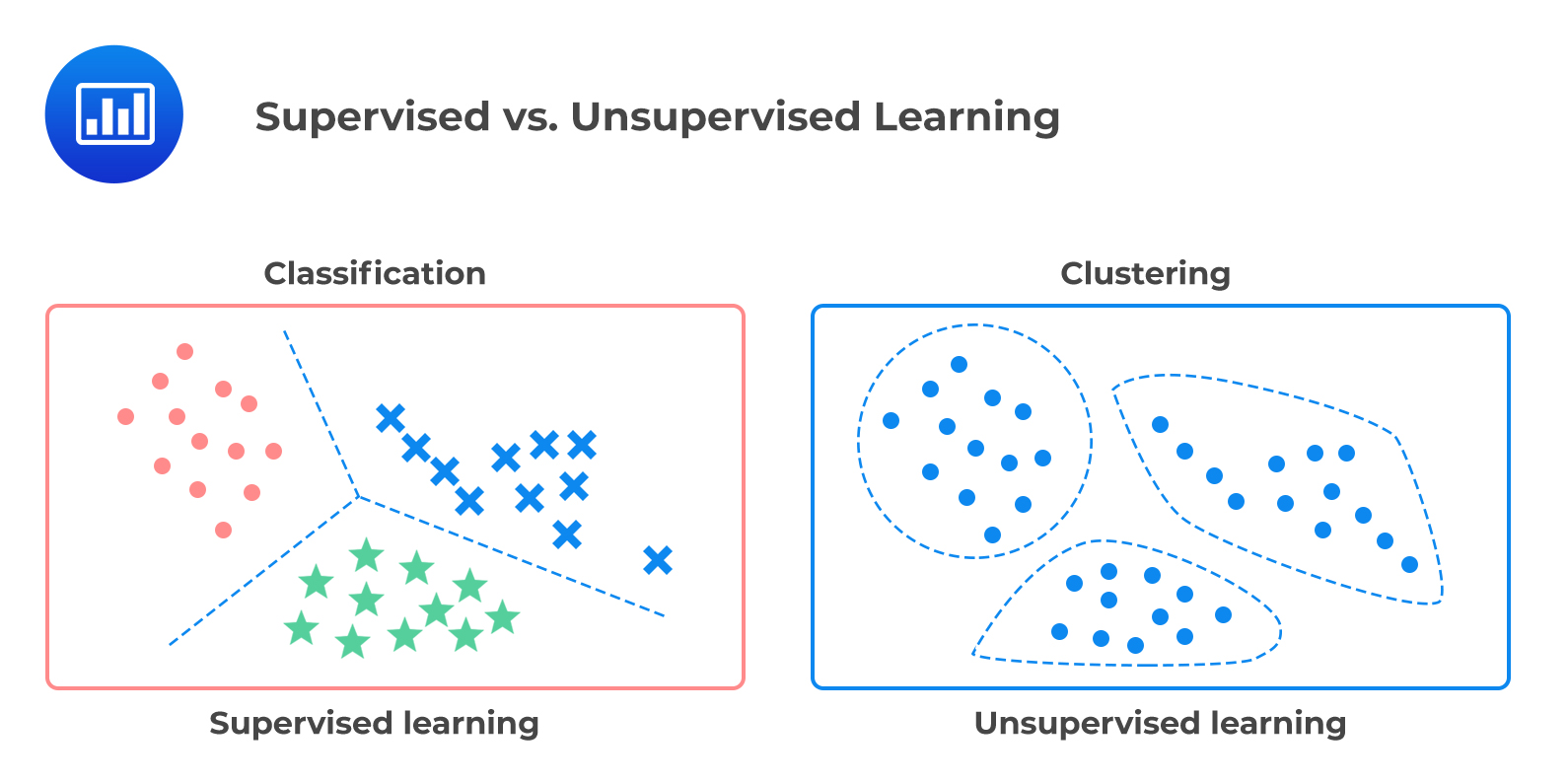
Supervised vs. Unsupervised Learning: Key Differences

While both supervised and unsupervised learning are valuable techniques, they serve different purposes. Here’s a summary of the key differences:

Feature	Supervised Learning	Unsupervised Learning
Input Data	Labeled data (input-output pairs)	Unlabeled data (no explicit outputs)
Goal	Predict outputs based on inputs	Find hidden patterns or structures
Examples	Classification, regression	Clustering, dimensionality reduction

Common Machine Learning Models and Their Real-Life Applications

Now that we’ve covered the basics of supervised and unsupervised learning, let’s take a closer look at some popular machine learning models used in real-life business applications. Each model has its strengths and is suited to different types of tasks.

1. Linear Regression

Linear Regression is one of the simplest and most widely used models for regression tasks. It models the relationship between a dependent variable and one or more independent variables by fitting a linear equation to the data.

Real-Life Example: In finance, linear regression is often used to predict stock prices based on historical data. By modeling the relationship between stock price and factors like market trends, economic indicators, and company performance, analysts can forecast future stock prices and make informed investment decisions.

2. Decision Tree

A Decision Tree is a tree-like structure where each node represents a decision based on a feature, and each branch represents the outcome of that decision. It is used for both classification and regression tasks.

Real-Life Example: In customer relationship management (CRM), decision trees are used to predict customer churn. By analyzing factors such as customer complaints, frequency of purchases, and customer satisfaction scores, decision trees help businesses understand which customers are likely to leave and why.

3. Random Forest

Random Forest is an ensemble learning method that builds multiple decision trees and merges their results to improve accuracy and prevent overfitting. It is effective for both classification and regression problems.

Real-Life Example: In the healthcare industry, Random Forest models are used to predict patient outcomes based on a range of medical data. By analyzing patient demographics, medical history, and lab results, Random Forest helps doctors make more accurate diagnoses and recommend personalized treatment plans.

4. XGBoost

XGBoost (Extreme Gradient Boosting) is a powerful and efficient boosting algorithm known for its high performance in both classification and regression tasks. It builds models sequentially, correcting errors from previous models to enhance overall accuracy.

Real-Life Example: In marketing, XGBoost is used for customer segmentation and personalized recommendations. By analyzing purchase history, browsing behavior, and demographic data, XGBoost models can predict which products a customer is likely to buy, enabling businesses to tailor their marketing campaigns effectively.

5. K-Nearest Neighbors (KNN)

The K-Nearest Neighbors (KNN) algorithm is a simple, instance-based learning model that classifies new data points based on the “k” closest points in the training set. KNN is often used for classification tasks.

Real-Life Example: In recommendation systems, KNN is used to suggest products or services to users based on similarities with other users. For example, Netflix uses KNN to recommend shows to users based on their viewing history and the preferences of similar users.

6. Support Vector Machines (SVM)

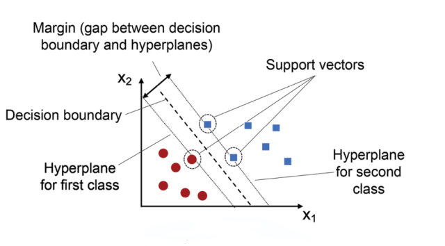
Support Vector Machines (SVM) are powerful supervised learning models used primarily for classification tasks. SVM works by finding the optimal hyperplane that separates the data into different classes.

Real-Life Example: In the finance industry, SVM is used for fraud detection. By analyzing patterns in transaction data, SVM models can detect anomalous behavior indicative of fraud and help financial institutions flag potentially fraudulent transactions.

7. K-Means Clustering (Unsupervised)

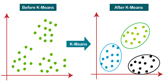
K-Means Clustering is one of the most popular unsupervised learning algorithms for partitioning data into clusters based on similarity. It is often used for grouping similar data points in large datasets.

Real-Life Example: In retail, K-Means clustering is used for customer segmentation. By analyzing purchase behavior, demographics, and shopping patterns, K-Means helps businesses group customers into distinct segments, enabling more targeted marketing efforts.

Conclusion

Understanding the differences between supervised and unsupervised learning and mastering model evaluation techniques is crucial for any data scientist or business looking to leverage machine learning effectively. Choosing the right model and evaluating it thoroughly ensures that the insights you derive are accurate and actionable.

Whether you’re trying to predict customer behavior using supervised learning or uncovering hidden customer segments with unsupervised learning, having a solid evaluation strategy in place will help you get the most out of your models and drive meaningful results for your business.

From predicting future trends with Linear Regression to uncovering hidden customer segments with K-Means, machine learning models offer powerful tools for solving a wide range of business problems. By understanding the strengths of each model, you can choose the best approach for your data and task at hand. And don’t forget, evaluating these models properly is key to ensuring that the insights they provide are accurate, reliable, and actionable.

Also, in this real world using supervised models like Decision Trees or unsupervised methods like K-Means clustering, machine learning is a vital asset for driving data-informed business strategies. As you continue to explore different models and applications, always prioritize model evaluation to ensure your results are both meaningful and scalable in real-world scenarios.

Stay tuned!