
Introduction
Outliers are a common issue
![]() data analysis and can significantly impact your results if not treated properly. Whether you’re working on sales data for a retail company or transaction data for a financial institution, outliers can skew your analysis and lead to incorrect conclusions. In this post, we will dive into what outliers are, how to identify them, and most importantly, how to treat them effectively.
data analysis and can significantly impact your results if not treated properly. Whether you’re working on sales data for a retail company or transaction data for a financial institution, outliers can skew your analysis and lead to incorrect conclusions. In this post, we will dive into what outliers are, how to identify them, and most importantly, how to treat them effectively.
What Are Outliers?
Outliers are data points that significantly differ from the rest of the dataset. They can arise due to various reasons, such as data entry errors, measurement inconsistencies, or even genuine anomalies. Outliers can either provide meaningful insights (e.g., fraudulent transactions) or distort your analysis (e.g., a typo in entered sales figures).
In real-life scenarios, think about how a small number of extremely high-priced items in an e-commerce store can skew the average price calculation. Identifying and treating outliers is essential to ensure that your analysis reflects the reality of the data.
The Role of Data Distribution
Before diving into how to treat outliers, it's important to understand the data distribution. Data distribution refers to the way data points are spread across different values. Understanding the distribution is crucial because it affects how we detect and treat outliers.
Types of Distributions
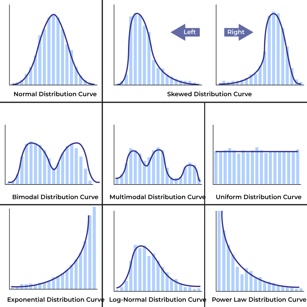
- Normal Distribution: Often referred to as a "bell curve," a normal distribution is symmetrical, with most of the data clustering around the mean. Outliers in a normal distribution are easier to spot because they occur at the tails.
- Skewed Distribution: Data is not evenly distributed. In right-skewed distributions, there are a few very large values (e.g., income levels in a population). In left-skewed distributions, the reverse is true. Skewness makes it harder to detect outliers because what may look like an outlier could simply be part of a long tail.
- Multimodal Distribution: This occurs when there are multiple peaks in the data. For example, test scores of students from different ability levels may form a multimodal distribution. Identifying outliers in this case can be complex.
Understanding the distribution of your data is crucial because it influences how we define and identify outliers. A data point that seems like an outlier in a normal distribution might not be one in a skewed distribution, and vice versa.
Visualizing Distributions
Before identifying outliers, it’s a good idea to visualize the distribution of your data. Some common ways to do this are:
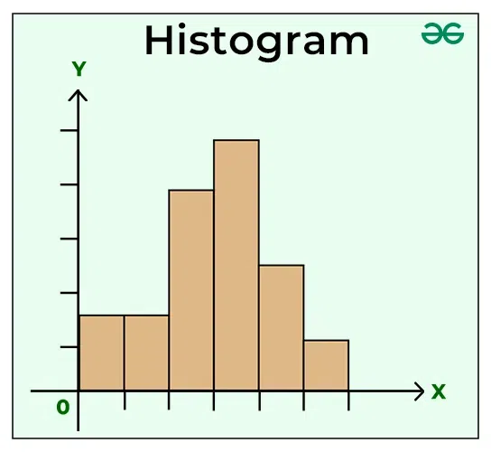
- Histograms:
A histogram is a bar chart that shows the distribution of your data. It’s a great tool for getting a sense of whether the data is normally distributed, skewed, or multimodal.
df['column_name'].hist(bins=30)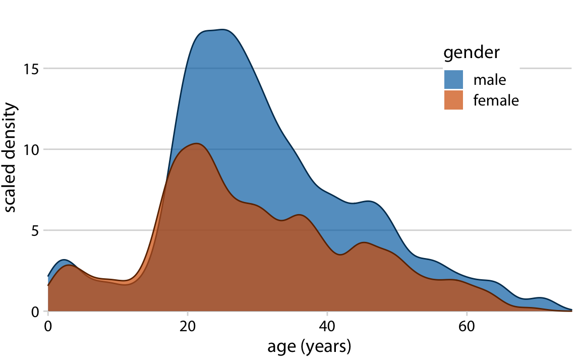
df['column_name'].plot(kind='density')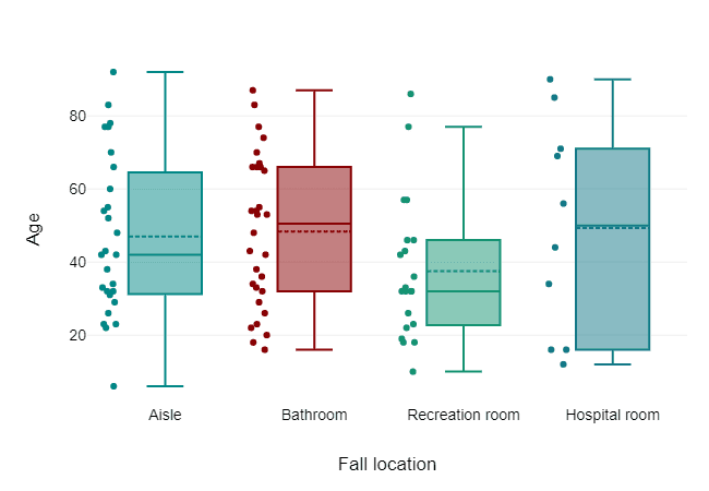
df.boxplot(column='column_name')Real-Life Example: Imagine you're analyzing the salaries of employees in a large corporation. If the data is normally distributed, most salaries will cluster around the average. However, if the distribution is skewed, with a few top executives earning significantly more than the average employee, this will create a right-skewed distribution. Knowing the type of distribution helps in accurately identifying whether the high salaries are outliers or just part of the expected spread.
Types of Outliers

There are two main types of outliers:
- Univariate Outliers: These are outliers that occur when looking at one variable at a time. For example, if most of the products in a store cost between $10 and $200, but one product is priced at $5,000, that would be a univariate outlier.
- Multivariate Outliers: These outliers occur in multidimensional datasets, where combinations of variables result in unusual data points. For example, if a user on a social media platform is engaging with a massive number of posts but is following very few accounts, that could be a multivariate outlier.
Identifying Outliers
Before treating outliers, we need to identify them. There are several methods to detect outliers in data:
1. Visualization Techniques

Boxplots: A boxplot is a great way to visualize outliers. It displays the distribution of the data and highlights points that fall outside the interquartile range (IQR).
df.boxplot(column='column_name')Scatter plots: Scatter plots can also help identify outliers, especially in multivariate data. By plotting two variables, we can see if any points fall far from the general cluster of data.
df.plot(kind='scatter', x='var1', y='var2')Real-Life Example: In the real estate industry, boxplots are often used to identify outliers in house prices. For example, if most houses in a neighborhood sell for $200,000 to $500,000, but there are a few properties priced at $2 million, those would be considered outliers.
2. Statistical Methods
Z-Score:
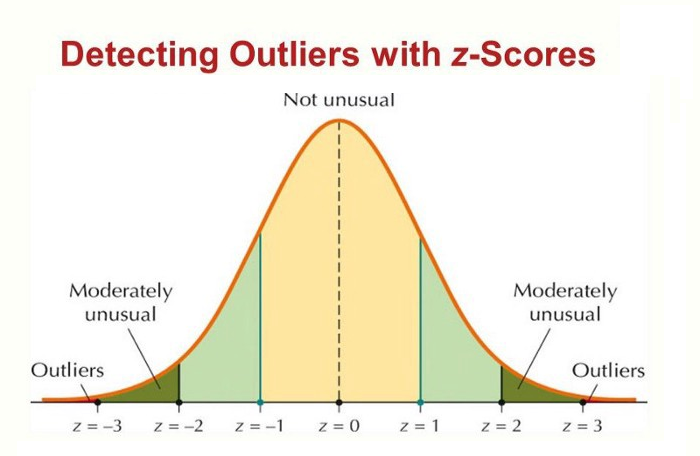
from scipy import stats
import numpy as np
z_scores = np.abs(stats.zscore(df['column_name']))
outliers = df[z_scores > 3]
Interquartile Range (IQR):
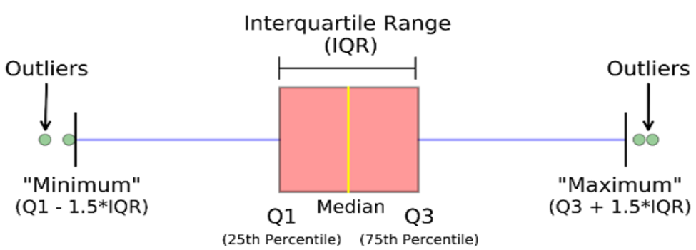
Q1 = df['column_name'].quantile(0.25)
Q3 = df['column_name'].quantile(0.75)
IQR = Q3 - Q1
outliers = df[(df['column_name'] < (Q1 - 1.5 * IQR)) | (df['column_name'] > (Q3 + 1.5 * IQR))]
Real-Life Example: In the stock market, traders often use Z-scores to detect outliers in stock prices. If a stock’s price moves more than three standard deviations from its average price, it could signal unusual activity or a potential trading opportunity.
Dealing with Outliers
Once outliers are identified, the next step is to decide how to treat them. There are several approaches, depending on the context and the nature of the outlier:
1. Removing Outliers
If the outliers are due to data entry errors or anomalies that don’t provide meaningful insights, it may be best to remove them. This can be done using the drop() function in Pandas.
df_cleaned = df[(z_scores < 3)]Real-Life Example: In an e-commerce platform like Amazon, if a product's price is accidentally entered as $0.01 instead of $10.01, it would be considered a data entry error and should be removed.
2. Transforming Outliers
If removing outliers isn't ideal, you can transform them. One popular method is to apply a log transformation to reduce the impact of extreme values. This is especially useful in skewed datasets.
df['log_transformed'] = np.log(df['column_name'] + 1)Real-Life Example: In finance, transaction amounts can vary widely. Applying a log transformation to transaction amounts can normalize the data, ensuring that extremely large transactions don’t disproportionately influence the analysis.
3. Imputation
Instead of removing outliers, you can replace them with more reasonable values. For example, you could replace an outlier with the mean or median value of the dataset.
df['column_name'] = np.where(df['column_name'] > upper_limit, df['column_name'].median(),
    df['column_name'])
Real-Life Example: In healthcare, outliers in patient data (e.g., extreme blood pressure readings) could be replaced with the median reading of other patients to avoid skewing the results of a study.
4. Binning

Binning involves categorizing continuous data into discrete bins. This method can be useful when you want to minimize the impact of outliers without completely discarding them.
df['binned_column'] = pd.cut(df['column_name'], bins=[0, 100, 200, 500, np.inf],
    labels=['Low', 'Medium', 'High', 'Very High'])
Real-Life Example: In a loyalty program at a retail store like Walmart, customers' purchase amounts can vary greatly. By binning customers into different categories based on their spending (e.g., low, medium, high), the store can target promotions to different groups without letting a few outliers (e.g., high spenders) affect the overall analysis.
Conclusion
Outliers are an unavoidable part of working with real-world data, but with the right techniques, they can be effectively managed. Whether you’re removing outliers, transforming them, or binning them into categories, it’s essential to understand the context of your data and choose the right method. In fields like finance, healthcare, and retail, understanding how to handle outliers can be the difference between gaining accurate insights and making flawed decisions.
In my next post, we’ll explore how to combine outlier detection with advanced machine learning techniques to build robust models.
Comments
Post a Comment